
USDA-NIFA Extension IPM Grant
Pest & Crop Newsletter, Entomology Extension, Purdue University
- Corn Grain Test Weight
- Corn Stalk Nitrate Tests - Research and Recommendation Update
- Purdue Economist Suggests Corn Growers Consider Keeping Their Crops Close to Home
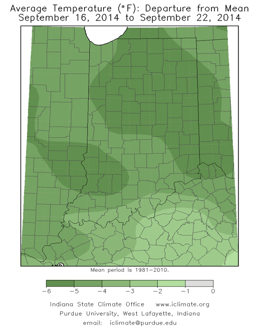
- October Weather Outlook: More Seasonal - For A Change
- Troubleshooting Corn Ear Abnormalities
- Assessing Yield Losses in Corn Due to Frost
Corn Grain Test Weight – (Bob Nielsen) -
Among the top 10 most discussed (and cussed) topics at hometown cafes during harvest season is the test weight of the grain being reported from corn fields in the neighborhood. Test weight is measured in the U.S. in terms of pounds of grain per volumetric bushel. In practice, test weight measurements are based on the weight of grain that fills a quart container (32 qts to a bushel) that meets the specifications of the USDA-FGIS (GIPSA) for official inspection (Fig. 1). Certain electronic moisture meters, like the Dickey-John GAC, estimate test weight based on a smaller-volume cup. These test weight estimates are reasonably accurate but are not accepted for official grain trading purposes.
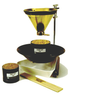
Fig 1. A standard filling hopper and stand for the accurate filling of quart or pint cups for grain test weight determination. (Image: http://www.seedburo.com)
The official minimum allowable test weight in the U.S. for No. 1 yellow corn is 56 lbs/bu and for No. 2 yellow corn is 54 lbs/bu (USDA-GIPSA, 1996). Corn grain in the U.S. is marketed on the basis of a 56-lb “bushel” regardless of test weight. Even though grain moisture is not part of the U.S. standards for corn, grain buyers pay on the basis of “dry” bushels (15 to 15.5% grain moisture content) or discount the purchase price to account for the drying expenses they will incur handling wetter corn grain.
Growers worry about low test weight because local grain buyers often discount the offered price paid to farmers for low test weight grain. In addition, growers are naturally disappointed when they deliver a 1000-bu semi-load of grain that averages 52-lb test weight because they only get paid for 929 56-lb “market” bushels (52,000 lbs ÷ 56 lbs/bu) PLUS they receive a discounted price for the grain. On the other hand, high test weight grain makes growers feel good when they deliver a 1000 bushel semi-load of grain that averages 60 lb test weight because they will get paid for 1071 56-lb “market” bushels (60,000 lbs ÷ 56 lbs/bu).
These emotions encourage a belief that high test weight grain (lbs of dry matter per volumetric bushel) is associated with high grain yields (lbs. of dry matter per acre) and vice versa. However, there is little evidence in the research literature that grain test weight has a strong positive relationship with grain yield.
Hybrid variability exists for grain test weight, but also does not necessarily correspond to differences in genetic yield potential. Grain test weight for a given hybrid often varies from field to field or year to year, but does not necessarily correspond to the overall yield level of an environment.
Similarly, grain from high yielding fields does not necessarily have higher test weight than that from lower yielding fields. In fact, test weight of grain harvested from severely stressed fields is occasionally higher than that of grain from non-stressed fields, as evidenced in Fig. 2 for 27 corn hybrids grown at 3 locations with widely varying yield levels in Kansas in 2011. Another example from Ohio with 22 hybrids grown in common in the drought year of 2012 and the much better yielding year of 2013 also indicated no effect of yield level on grain test weight (Fig. 3).
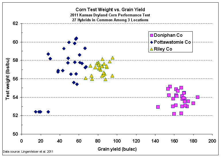
Fig 2. Corn grain test weight versus grain yield for 27 hybrids grown at 3 Kansas locations (Lingenfelser et al, 2011)
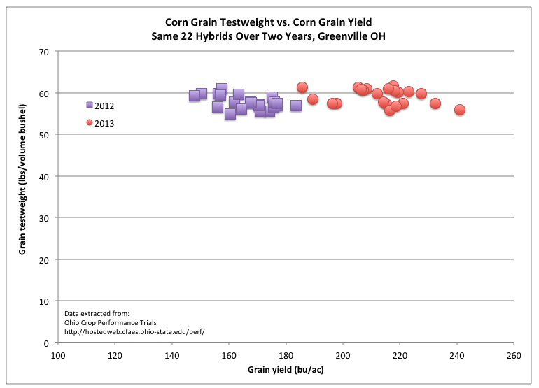
Fig 3. Corn grain test weight versus grain yield for 22 hybrids frown at Greenville, OH in 2012 (drought) and 2013 (ample rainfall)
Conventional dogma suggests that low test weight corn grain decreases the processing efficiency and quality of processed end-use products like corn starch, although the research literature does not consistently support this belief. Similarly, low test corn grain is often thought to be inferior for animal feed quality, although again the research literature is not in agreement on this. Whether or not low test weight grain is inferior to higher test weight grain may depend on the cause of the low test weight in the first place.
Common Causes of Low Grain Test Weight
Back in the 2009 harvest season in Indiana, there were more reports of low test weight corn grain than good or above average test weights. There were primarily six factors that accounted for most of the low test weight grain in 2009 and four shared a common overarching effect.
Grain Moisture
First and foremost, growers should understand that test weight and grain moisture are inversely related. The higher the grain moisture, the lower the test weight. As grain dries in the field or in the dryer, test weight naturally increases as long as kernel integrity remains intact. Test weight increases as grain dries partly because kernel volume tends to shrink with drying and so more kernels pack into a volume bushel and partly because drier grain is slicker which tends to encourage kernels to pack more tightly in a volume bushel.
Therefore in a year like 2009 with many of the initial harvest reports of grain moisture ranging from 25 to 30% instead of the usual starting moisture levels of about 20 to 23%, it should not be surprising that test weights were lower than expected. Hellevang (1995) offered a simple formula for estimating the increase in test weight with grain drying. In its simplest form, the equation is (A/B) x C; where A = 100 - dry moisture content, B = 100 - wet moisture content, and C = test weight at wet moisture content. The author does not say, but I suspect this simple formula is most applicable within a “normal” range of harvest moistures; up to moistures in the mid- to high 20’s.
Example: Dry moisture = 15%, Wet moisture = 25%, Test weight at 25% = 52 lbs/bu.
Estimated test weight at 15% moisture = ((100 - 15) / (100 - 25)) x 52 = (85/75) x 52 = 58.9 lbs/bu
An older reference (Hall & Hill, 1974) offers an alternative suggestion for adjusting test weight for harvest moisture that also accounts for the level of kernel damage in the harvested grain (Table 1). The table values are based on the premise that kernel damage itself lowers test weight to begin with and that further drying of damaged grain results in less of an increase in test weight that what occurs in undamaged grain. Compared to the results from using Hellevang’s simple formula, adjustments to test weight using these tabular values tend to result in smaller adjustments to test weight for high moisture grain at harvest, but larger adjustments for drier grain at harvest.
| Table 1. Adjustment added to the wet-harvest test weight to obtain an expected test weight level after drying to 15.5 percent moisture. | ||||||||
| Percent Damage |
Grain Moisture at Harvest (Percent) | |||||||
| 30 | 28 | 26 | 24 | 22 | 20 | 18 | 16 | |
| 45 | 0.3 | |||||||
| 40 | 0.7 | 0.2 | ||||||
| 35 | 1.3 | 0.7 | ||||||
| 30 | 1.8 | 1.3 | 0.8 | |||||
| 25 | 2.4 | 1.9 | 1.4 | 0.9 | 0.3 | |||
| 20 | 3.1 | 2.6 | 2.0 | 1.5 | 1.0 | 0.5 | ||
| 15 | 3.8 | 3.2 | 2.7 | 2.2 | 1.7 | 1.2 | 0.6 | 0.2 |
| 10 | 4.5 | 4.0 | 3.5 | 2.9 | 2.2 | 1.9 | 1.4 | 0.8 |
| 5 | 5.3 | 4.7 | 4.2 | 3.7 | 3.0 | 2.7 | 2.1 | 1.6 |
| 0 | 6.1 | 5.6 | 5.0 | 4.5 | 4.0 | 3.5 | 2.9 | 2.4 |
| Source: Hall & Hill, 1974 | ||||||||
Stress During Grain Fill
Secondly, thirdly, and fourthly; drought stress, late-season foliar leaf diseases (primarily gray leaf spot and northern corn leaf blight), and below normal temperatures throughout September of 2009 all resulted in a significant deterioration of the crop’s photosynthetic machinery beginning in early to mid-September that “pulled the rug out from beneath” the successful completion of the grain filling period in some fields; resulting in less than optimum starch deposition in the kernels. Fifthly, early October frost/freeze damage to late-developing, immature fields resulted in leaf or whole plant death that effectively put an end to the grain-filling process with the same negative effect on test weight.
Ear Rots
Finally, there were widespread reports of ear rots (diplodia, gibberella, etc.) throughout many areas of Indiana in 2009. Kernel damage by these fungal pathogens results in light-weight, chaffy grain that also results in low test weight diseased grain, broken kernels, and excessive levels of foreign material. This cause of low test weight grain obviously results in inferior (if not toxic) animal feed quality grain, unacceptable end-use processing consequences (ethanol yield, DDGS quality, starch yield and quality, etc.), and difficulties in storing the damaged grain without further deterioration.
Related References
Bern, Carl and Thomas Brumm. 2009. Grain Test Weight Deception. Iowa State Extension Publication PMR-1005. [online] <http://www.extension.iastate.edu/Publications/PMR1005.pdf>. [URL accessed Sep 2014].
Bradley, Carl. 2009. Diplodia Ear Rot Causing Problems in Corn Across the State. The Bulletin, Univ of Illinois Extension. [online]. <http://ipm.illinois.edu/bulletin/article.php?id=1233>. [URL accessed Sep 2014].
Hall, Glenn and Lowell Hill. 1974. Test Weight Adjustment Based on Moisture Content and Mechanical Damage of Corn Kernels. Trans. ASAE 17:578-579.
Hellevang, Kenneth. 1995. Grain Moisture Content Effects and Management. North Dakota State Extension Publication AE-905. [online]. <http://www.ag.ndsu.edu/extension-aben/documents/ae905.pdf>. [URL accessed Sep 2014].
Hicks, D.R. and H.A. Cloud. 1991. Calculating Grain Weight Shrinkage in Corn Due to Mechanical Drying. Purdue Extension Publication NCH-61 [online]. <http://www.ces.purdue.edu/extmedia/nch/nch-61.html> [URL accessed Sep 2014].
Hill, Lowell D. 1990. Grain Grades and Standards: Historical Issues Shaping the Future. Univ. of Illinois Press, Champaign, IL.
Hurburgh, Charles and Roger Elmore. 2008. Corn Quality Issues in 2008 - Moisture and Test Weight. Integrated Crop Management News, Iowa State Univ. Extension. [online]. <http://www.extension.iastate.edu/CropNews/2008/1023hurburghrobertsonelmore1.htm>. [URL accessed Sep 2014].
Hurburgh, Charles and Roger Elmore. 2008. Corn Quality Issues in 2008 – Storage Management. Integrated Crop Management News, Iowa State Univ. Extension. [online]. <http://www.extension.iastate.edu/CropNews/2008/1023hurburghrobertson.htm>. [URL accessed Sep 2014].
Lingenfelser, Jane (sr. author). 2011. Kansas Crop Performance Tests with Corn Hybrids (SRP1055). Kansas State University Agricultural Experiment Station and Cooperative Extension Service, Kansas State Univ.
Nafziger, Emerson. 2003. Test Weight and Yield: A Connection? The Bulletin, Univ of Illinois Extension. [online]. <http://ipm.illinois.edu/bulletin/pastpest/articles/200323h.html>. [URL accessed Sep 2014].
USDA-GIPSA. United States Standards for Corn. 1996. USDA Grain Inspection, Packers and Stockyards Administration (GIPSA). [online] <http://www.gipsa.usda.gov/fgis/standards/810corn.pdf>. [URL accessed Sep 2014].
Wise, Kiersten and Charles Woloshuk. 2009. Dealing With Diplodia Ear Rot. Pest & Crop Newsletter, Purdue Extension. [online]. <http://extension.entm.purdue.edu/pestcrop/2009/issue24/index.html>. [URL accessed Sep 2014].
![]()
Corn Stalk Nitrate Tests – Research and Recommendation Update - (Jim Camberato and Bob Nielsen) -
The corn stalk nitrate test (CSNT) can be used as an end-of-season assessment of a nitrogen (N) management program relative to N source, timing, placement, and rate (Brouder, 2003). For this diagnostic test, 15 or more 8-inch stalk segments (beginning 6 inches above the soil surface) are taken from representative areas of a field from about two weeks prior to or 3 weeks after kernel black layer formation and analyzed for nitrate- nitrogen (NO3-N). Accumulation of NO3-N in the lower corn stalk results from N availability exceeding crop N utilization.
Timing of corn stalk sampling
Although stalk samples are typically collected within two to three weeks after black layer formation in accordance with the guidelines initially suggested by Iowa researchers (Binford et al., 1990), there is interest in assessing N management for silage corn which is harvested prior to black layer. Pennsylvania researchers compared results and interpretation of corn stalk NO3-N samples taken at ¼ milk line (milk line positioned about 25% of the distance from the dented crown to the kernel tip) to those obtained 1 to 3 weeks after black layer (Fox et al., 2001). Stalk NO3-N levels did not differ among samples taken between ¼ milk line and 1 to 3 weeks after black layer for 176 of 209 comparisons. Where differences occurred, there was no strong trend in the direction of change; 20 increased and 13 decreased from ¼ milk line to black layer. The researchers concluded that the interpretation of the CSNT in Pennsylvania was the same for samples obtained beginning at ¼ milk line through a few weeks after black layer (Beegle and Rotz, 2009).
Interpretation of corn stalk NO3-N concentrations
Previous research conducted in Indiana in 1996 and 1997 concluded that NO3-N concentrations less than 450 ppm were low, between 450 and 2,000 ppm were associated with optimal N availability, while concentrations greater than 2,000 ppm NO3-N indicated N availability was excessive (Brouder, 2003). The relationship between corn stalk NO3-N and relative yield from our more recent 35 site-years of N response trials conducted in 2007-2009 and 2011-2013 (Fig. 1) are similar to earlier findings, suggesting similar interpretations are relevant for modern hybrids. Most of our studies were conducted with at-planting or sidedress N application of 28% urea-ammonium nitrate. Although the timing and form of N were not found to alter the relationship between corn stalk NO3-N in earlier Iowa and Indiana research, recent research conducted in Iowa (Kyveryga and Blackmer, 2013) suggests the fall application of manure may need to be evaluated differently (discussed later).
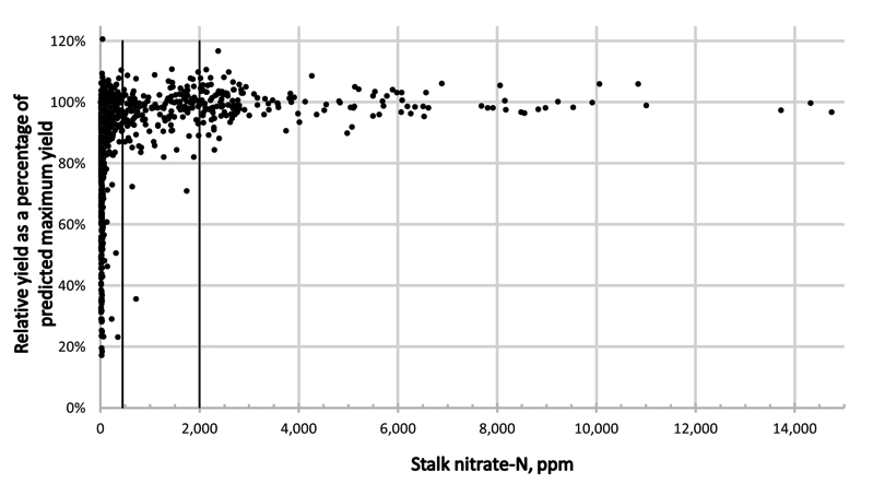
Fig 1. Stalk nitrate-N relationship with relative yield for 35 site-years of N trials conducted in Indiana from 2007-2009 and 2011-2013. Within each location and year the yield of an individual N rate treatment was related to the predicted maximum yield at the location in that year. The vertical bars indicate the divisions between low, optimal, and excessive levels as originally defined by Brouder (2003)
Previous Indiana guidelines did not attempt to quantify the relationship between corn stalk NO3-N concentrations and deficit or surplus levels of N fertilization. Thus specific recommendations on how much to increase or decrease N fertilization were not made. In attempt to make more specific recommendations on how to alter N fertilization rates based on corn stalk NO3-N concentrations, the recently collected Indiana data were categorized by corn stalk NO3-N and and compared to relative yield and the difference in fertilizer N rate relative to the N rate needed to obtain maximum yield.
Low corn stalk NO3-N: Less than 251 ppm
Sixty-three percent of corn stalk samples had
N03-N concentrations less than 251 ppm (Table 1). Relative grain yield in this low NO3-N category ranged from less than 20 to greater than 100% of maximum yield (Figure 1) and averaged 81%. Almost all relative yields less than 80% of maximum yield were associated with corn stalk NO3-N concentrations less than 251 ppm (Figure 1). However, 17% of corn stalk NO3-N concentrations less than 251 ppm wer associated with N rate tratments producing 98 to more than 100% of maximum yield. Therefore, low corn stalk NO3-N does not always mean the crop was short of N.
| Table 1. Relative yield (as % of predicted maximum yield within each of 35 location-years) and N rate deficit (-) or excess (+) (relative to the N rate needed to maximize yield in that location-year) for various categories of end-or-season corn stalk NO3-N. Individual data points are shown in Fig. 1. | |||
| Corn stalk NO3-N, ppm | Relative % yield | N deficit (1) or excess (+), pounds per acre | Number of observations |
| ≤250 | 81 | -92 | 661 |
| 251 - 500 | 96 | -27 | 61 |
| 501 - 1,000 | 96 | -24 | 65 |
| 1,001 - 1,500 | 98 | -9 | 45 |
| 1501 - 2,000 | 99 | 5 | 45 |
| 2001 - 4,000 | 100 | 33 | 110 |
| 4,001 - 8,000 | 99 | 53 | 38 |
| >8000 | 100 | 77 | 16 |
Optimal corn stalk NO3-N: From 251 to 2,000 ppm
Twenty-one percent of corn stalk samples had NO3-N concentrations between 251 and 2,000 ppm, which is categorized as optimal. All but 3 of 216 observations in this category had relative yields greater than 80% (Figure 1). At the lower end of this category, between 251 and 500 ppm NO3-N, average relative yield was 96% and the average N fertilizer deficit was 27 lb N/acre (Table 1). At the upper end of the optimal category, 1,501-2,000 ppm NO3-N, average relative yield was 99% and an average fertilizer surplus of 5 lb N/acre occurred.
Recommended N fertilizer rates target maximum profit, not maximum yield, thus they are lower than N rates needed to achieve maximum yield. At a commonly occurring corn grain to pound of N price ratio of 10 to 1 [grain at $4/bushel and N at $0.40/lb N ($225/ton 28% UAN)], economic optimum N fertilization rates are approximately 15 to 20 lb N/acre less than those needed to obtain maximum yield (Camberato et al., 2014). Therefore, corn stalk NO3-N levels between 1,000 and 2,000 ppm on average represent economically optimum N fertilization rates.
Excessive corn stalk NO3-N: Greater than 2,000 ppm
Eleven percent of corn stalk samples had NO3-N concentrations between 2,001 and 4,000 ppm. Average relative yield was 100% and average excess N was 33 lb N/acre.
Although it would be ideal to apply the optimum fertilizer N rate every year, it is not likely to happen. Based on our field-scale research, plus or minus 30 lb N/acre is a normal variation for optimum N rate from year to year for a particular cropping system. Although one year with corn stalk NO3-N between 2,001 and 4,000 ppm does not necessarily warrant a change in N management, multiple years at this level indicate the chosen N rate is higher than necessary for achieving maximum yield, as well as profit, and a reduction in N rate is suggested.
Corn stalk NO3-N concentrations between 4,000 and 8,000 ppm represented 4% of the samples obtained and were associated with excess N applications averaging 53 pounds per acre greater than that needed to achieve maximum yield (Table 1). Less than 2% of corn stalk samples had NO3-N greater than 8,000 ppm. The average excess N application was 77 pounds of N per acre for this category.
Corn stalk NO3-N concentrations in excess of 4,000 ppm represent excessive N application rates substantially beyond what is needed to obtain maximum yield or profit and reductions in N application rate should be strongly considered.
Using the end-of-season corn stalk nitrate test to adjust fertilizer-based N management programs
Multiple seasons of CSNT evaluation are warranted before altering a fertilizer N management program because the optimum N rate for a specific field can easily vary plus or minus 30 lb N/acre from season to season. Many factors affect the optimum N rate; including soil N supply, loss of N from the root zone, hybrid differences for N use, pest and weed impacts on N use, and the interaction of these and other factors. Thus the evaluation of a N management system with the CSNT (or any other N assessment tool) on any given field in a single season is interesting, but not particularly useful in making management decisions for future years. Unfortunately, there is no clear guidance on how many years the CSNT should be conducted, but three or more seasons are probably reasonable.
If end-of-season corn stalk NO3-N concentrations are consistently less than 250 ppm or more than 2,000 ppm one might consider conducting N response strip trials to identify the optimum N rate, rather than rely solely on the CSNT to alter the current N management program. Guidelines for conducting field-scale N response trials are available online (Nielsen and Camberato, 2011).
Manure-based N management programs and the corn stalk nitrate test
Recent research suggests the current interpretations of optimal and excessive N may be incorrect when fall-applied manure is the N source. Results of 52 trials with fall-applied manure showed that when corn stalk NO3-N was 3,500 ppm or less there was a greater than 50% probability of having had a profitable response to additional N (Kyveryga and Blackmer, 2013). Conducting strip trials to assess N response in manure-based N management programs would definitely be encouraged in light of these findings.
Interestingly this Iowa research with fall, spring, or sidedress fertilizer applications found a 50% probability of a response to additional N occurred at 500 ppm; well within the current interpretations used in Iowa and Indiana.
Related References
Beegle, D. and J. Rotz. 2009. Late season cornstalk nitrate test. Penn State Univ. Agronomy Facts 70. <http://nmplans.net/LateSeasonCornstalkNitrateTest.pdf> [URL accessed Sept 2014].
Binford, G.D., A.M. Blackmer, and N.M. El-Hout. 1990. Tissue test for excess nitrogen during corn production. Agronomy Journal 82:124-129
Brouder, Sylvie. 2003. Cornstalk testing to evaluate the nitrogen status of mature corn: Nitrogen management assurance. Purdue University Coop. Ext. publication AY-322-W. <http://www.agry.purdue.edu/ext/pubs/AY-322-W.pdf> [URL accessed Sept 2014].
Camberato, J., R.L. (Bob) Nielsen, and B. Joern. 2014. Nitrogen management guidelines for corn in Indiana. J. Camberato, R.L. Nielsen, and B. Joern. Applied Crop Research Update, Purdue Univ. Agronomy Dept. <http://www.kingcorn.org/news/timeless/NitrogenMgmt.pdf> [URL accessed Sept 2014].
Fox, R.H., W.P. Piekielek, and K.E. Macneal. 2001. Comparison of late-season diagnostic tests for predicting nitrogen status of corn. Agronomy Journal 93:590–597.
Kyveryga, Peter and Tracy M. Blackmer. 2013. 4R management: Differentiating nitrogen management categories on corn in Iowa. Better Crops/Vol. 97 (No. 1) 4-6. <http://goo.gl/uYLRgR> [URL accessed Sept 2014].
Nielsen, Bob and Jim Camberato. 2011. Purdue On-Farm Nitrogen Rate Trial Protocol.
Agronomy Dept, Purdue Univ. <http://www.agry.purdue.edu/ext/ofr/protocols/PurdueNTrialProtocol.pdf> [URL accessed Sept 2014].
We gratefully acknowledge the support provided for these trials by the Indiana Corn Marketing Council, Pioneer Hi-Bred Int’l and LG Seeds (seed contribution for Purdue trial sites), A&L Great Lakes Labs (discounted analysis costs), individual farmers and crop consultants, Purdue Univ. Office of Ag Research Programs, and all of the Purdue Ag Center staff.
![]()
Purdue Economist Suggests Corn Growers Consider Keeping Their Crops Close to Home – (Darrin Pack, Ag Answers)
With a record amount of corn likely headed to market in the next few weeks and corn prices still very low, a Purdue University agricultural economist is advising growers to consider storing their crop on their own property if they can.
The alternatives are to pay a premium for space in a commercial storage facility or to sell for prices far below what many farmers expected at the beginning of the season, said associate professor Corinne Alexander.
None of these three options is particularly appealing, Alexander says, but keeping the crops in on-farm bins, elevators or silos and waiting for market conditions to improve makes the most financial sense.
“If you don’t have storage on your farm, your next best choice might be to sell even if you have to take less than you wanted,” she said. “It’s a complex equation and there are no easy answers.”
Typically, the key variable in determining whether to store or sell crops is the “opportunity cost,” Alexander said. That is, farmers should calculate whether they would earn more by depositing the proceeds of an immediate sale or by storing their crops and hoping for higher prices later on.
But historically low interest rates right now mean farmers probably won’t lose much, if anything, by keeping their grain in silos instead of money in the bank, Alexander said.
Farmers also should consider that this year’s corn glut is likely to quickly fill up the region’s grain storage units, making space harder to find and more expensive, Alexander said.
“Indiana has done a good job in recent years of adding more storage space,” she said. “But with so much corn coming in at once it will be difficult to find room for it all.”
Alexander envisions a situation where excess corn could be “sitting around in piles” while producers and buyers try to figure out what to do with it.
But Indiana is unlikely to experience the types of transportation logjams facing farmers in the Dakotas. Analysts from the public and private sectors say the state has enough rail cars and barges to move the grain.
The questions are where will the buyers be found, at what prices and when?
With such a large surplus, Alexander said, corn prices are unlikely to recover their relatively high levels of the past two years anytime soon.
Corn prices have been battered since mid-summer when it became apparent that cool, wet weather would provide ideal conditions for a bumper crop.
The latest U.S. Department of Agriculture crop production report, issued Sept. 11, projected a record national corn output this year of 14.4 billion bushels, up 3 percent from 2013. Indiana farmers also were expected to produce a record crop.
As a result, the December corn contract, the most actively traded in the futures market, peaked at $5.10 per bushel in mid-May and has since slid to its lowest level in four years. Prospects for the basis price - the cash value farmers receive for the immediate sale of their crop at the time of harvest - are equally bleak because of the massive amount of grain up for sale.
Meanwhile, global demand for corn has plateaued, at least for the short term, due in part to a healthy wheat harvest in Europe that reduced their need for American grain imports and record or near-record production in other corn-growing countries.
Domestic demand is limited by barriers to growth in the ethanol and livestock feed sectors, two of the most important destinations for Indiana corn. Ethanol producers are using about all the corn they can for the foreseeable future, and livestock operators are just now beginning to increase their herds after several down years, Alexander said.
The good news, Alexander said, is American consumers might pick up some of the slack.
“If corn is cheap,” she said, “people will find ways to use it.”
![]()
October Weather Outlook: More Seasonal - For a Change - (Keith Robinson, Ag Answers) -
After an unusually cool and wet summer, Indiana might very well see a return to more normal conditions as autumn sets in.
Temperatures are expected to rebound to near-normal and then normal for the rest of September and develop into a warmer-than-normal trend for October, according to the Indiana State Climate Office, based at Purdue University. Precipitation should be about normal in October.
The relative warm-up would be the result of a “positive” Arctic Oscillation that is expected to keep cooler air out of the region and a jet stream that is likely to shift more east to west than north to south.
The outlook is “a broad climatology of expectations,” said Dev Niyogi, state climatologist.
“This appears to be a season where we will have to keep a close eye to see how things are evolving every month, with no major drivers dominating our seasonal outlook,” he said.
From now to the end of October in the far northern counties, daily high temperatures normally fall from 70°F to 55°F and lows from 50° to 40°F. In extreme southwest Indiana, the highs normally cool from 78° to 64° and the lows from 54° to 42°F.
Total October precipitation normally ranges between 1.7 and 1.9 inches across the state. October usually is one of the driest months of the year in Indiana.
With autumn’s return, attention shifts to the question of when Indiana will have its first frost. The average earliest first-frost dates are more than three weeks away.
For most of Indiana, the first killing freeze of 28°F or lower typically has occurred during of period of Oct. 23-29. Scattered portions of the state, mostly in some of the central and northern counties, have had their first frost Oct. 17-23.
Most southern counties have experienced their first frost Oct. 29 to Nov. 17.
A map of Indiana’s average first-frost dates is available at <http://www.iclimate.org/images/toolbox/Fall28.jpg>.
![]()
Troubleshooting Corn Ear Abnormalities – (Peter Thomison, Alley Geyer, and David Lohnes, The Ohio State University) -
When checking corn fields prior to and during harvest it’s not uncommon to encounter abnormal corn ears such as those shown above (Fig.1), especially when the crop has experienced stress conditions. Some of these abnormalities affect yield and grain quality adversely. We recently updated “Troubleshooting Abnormal Corn Ears” (available online at <http://u.osu.edu/mastercorn/>) to help corn growers and agricultural professionals diagnose and manage various ear and kernel anomalies and disorders.
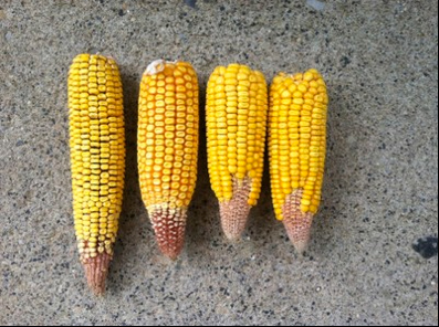
Fig. 1. Corn ears exhibiting "tip dieback", S. Charleston, OH 2014.
Also available is a poster (Fig. 2) highlighting ten abnormal corn ears with distinct symptoms and causes. The purpose of the poster is to help troubleshoot various ear disorders. A reduced 11 x 14 inch version of the poster is available for online at:
<http://agcrops.osu.edu/specialists/corn/specialistannouncements/AbnormalCornEarsPoster_000.pdf/view>
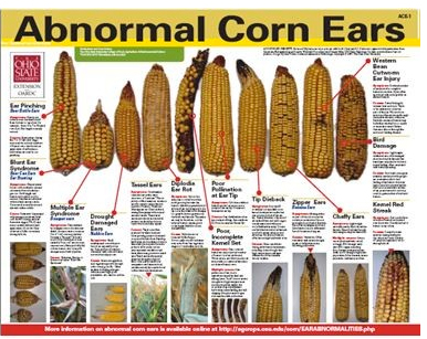
Fig. 2. "Abnormal Corn Ears" poster ACE-1
The OSU College of Food Agric. and Env. Sci. Communications & Technology section (contact information below) has 26 x 33 inch copies of the poster available for distribution. The poster is printed on plasticized coated paper for durability. Poster cost is $11.25 plus shipping. Ask for “Abnormal Corn Ears” poster” ACE-1.
The OSU College of Food Agric. and Env. Sci. Communications & Technology section (contact information below) has 26 x 33 inch copies of the poster available for distribution. The poster is printed on plasticized coated paper for durability. Poster cost is $11.25 plus shipping. Ask for “Abnormal Corn Ears” poster” ACE-1.
The Ohio State University
College of Food Agric. & Env. Sci.
Communications and Technology
Media Distribution
216 Kottman Hall, 2021 Coffey Road
Columbus, OH 43210-1044
E-mail: <pubs@ag.osu.edu>
Order Online: <http://estore.osu-extension.org/>
Phone: 614-292-1607
Fax: 614-292-124
![]()
With scattered frosts predicted in parts of Ohio tonight, it may be time to consider the impact of frost injury to corn that has not yet achieved kernel �black layer�. Black layer is the stage at which kernel growth ceases and maximum kernel dry weight is achieved (also referred to as �physiological maturity�). According to the USDA/NASS
For those growers with questions on the impact of frost damage on grain yield and maturation, one good source of information is �Handling Corn Damaged by Autumn Frost� NCH-57 by P.R.Carter and O. B. Hesterman available online at
. This publication includes information on the effect of frost on grain development and describes options for handling damaged corn. The following is an excerpt from the publication that addresses effects of frost injury on yield potential and whole plant and kernel moisture.�
The effect of frost damage to corn depends on the severity of defoliation, stalk damage, and stage of growth. Tables 1 and 2 provide yield loss and kernel moisture estimates resulting from premature plant death during grainfill. The tables summarize the findings of Minnesota researchers who defoliated plants to simulate frost damage at different kernel development stages.
| Table 1. Yield Loss in Corn as a Result of Plant Defoliation at Three Kernel Development Stages | |
| Kernel Development Stage | Percent Grain Yield Reduction |
| Soft dough | 34-36 |
| Full dent | 22-31 |
| Late dent | 4-8 |
| Source: Afuakwa, J.J., and R.K. Crookston. 1984. Using the kernel milklie to visually monitor grain maturity in maize. Crop Science 24: 687-691. | |
| Table 2. Whole Plant and Kernel Moisture of Corn at Four Kernel Development Stages | ||
| Kernel Development Stage | Kernel | Whole Plant |
| Percent Moisture | ||
| Soft dough | 62 | >75 |
| Full dent | 55 | 70 |
| Late dent | 40 | 61 |
| Physiological magturity (Black Layer*) | 32 | 53 |
*Black Layer - indicates end of kernel growth and maximum kernel dry weight (physiological maturity) |
||
| Source: Afuakwa, J.J., and R.K. Crookston. 1984. Using the kernel milkline to visually monitor grain maturity in maize. Crop Science 24: 687-691. | ||
![]()
Starting Next Year Now: The Utility of Fall Herbicide Applications – (Travis Legleiter and Bill Johnson) -
The 2014 harvest season has started and should be in high gear within the next week. As producers begin harvest they will need to be thinking about many management plans for next seasons crop. Herbicide programs and weed management strategies will be one of those topics that producers need to consider this fall as harvest wraps up this current growing season.
Fall herbicide applications should be considered by Indiana’s no-till farmers, especially those who have had past problems with marestail. The focus of a fall application for most winter annual weeds should be to control the weeds that are present in the field in the fall rather than plants that will emerge next spring. This fall is likely to give us a lot of winter annual weed emergence since we have had high amounts of precipitation in August and September. In most cases, a properly timed application of glyphosate, 2,4-D, and/or dicamba from mid-October to mid-November will control the weeds that emerged this fall and provide fields with lower densities of smaller weeds next spring that can be more easily controlled with a spring burndown, than fields that did not receive a fall burndown.
The necessity of a residual herbicide in the fall is always in debate amongst producers and weed scientists. A residual herbicide applied later in the fall can keep fields cleaner longer in the spring, and can in some years provide enough activity to keep fields clean up to planting. With the cold, harsh winter we experienced this past fall, residual herbicides persisted well into the spring planting season. There were several cases this year where residuals persisted too long and soybean injury occurred because of additive effects from the remnant fall residual and a spring residual that was applied. The success of this past years fall residual herbicides will not occur every year, it all depends on the weather and we all know it’s improbable to predict what the winter and next spring will bring. In a year with a warmer than usual winter and early spring the residuals will quickly break down and allow winter annuals to emerge into the planting season, which will require another burndown and another residual herbicide to control weeds into the soybean growing season. This is why our general recommendation from year to year is to save the residual until the spring when you know that it will persist into the soybean-growing season.
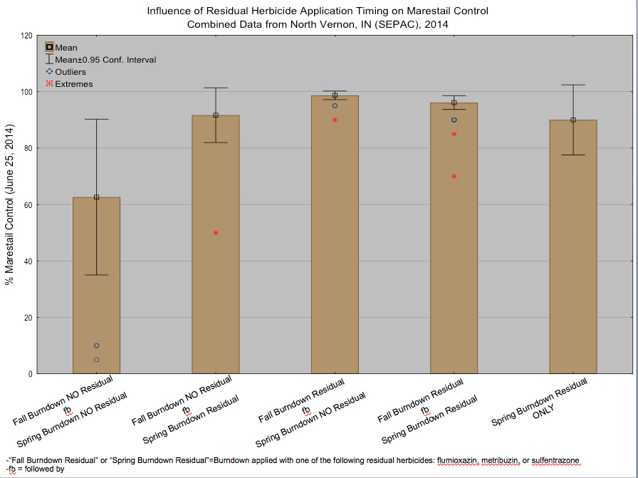
Influence of residual herbicide application timing on marestail control
The recommendation from Purdue has been and will remain to be that fall applications should consist of products that will control the weeds that are present and to save the use of a residual herbicide until as close to planting as possible in the spring. This eliminates the guessing game of what the winter and spring will bring and whether of not an additional residual application will be needed. A planned fall burndown without residual followed by a spring burndown with residual assures that the residual will still be present into the growing season. However, given our continual struggle to control marestail throughout much of the state, we are revising this recommendation in areas where additional horsepower is needed for marestail control.
The use of a fall application, regardless of whether or not it includes a residual, is a must if you are trying to control marestail in no-till soybean. The emergence pattern of marestail in fall as well as in the spring and summer means that multiple herbicide applications are needed and these applications need to start in the fall. Again the fall application needs to focus primarily on controlling the marestail rosettes that emerged in the fall and we will like to see a low-cost residual component added to the foliar product. The residual component should not be expected to provide residual control of marestail in the spring for more than 2 weeks. A program like this will make the spring burndown more effective as there will be less marestail plants to control and the plants present will be the smaller spring emerged rosettes, rather than large bolting fall-emerged plants.
The included chart shows the need not only for multiple burndown applications, but also the need for residual herbicides to effectively manage marestail in no-till soybean. The data in the chart was collected from treatments applied at the Southeast Purdue Agriculture Center in North Vernon, IN during this previous growing season. Treatments were grouped by when applications were made and whether or not they included one of the following residual herbicides that are recommended by Purdue for marestail control: flumioxazin (Valor), sulfentrazone (Authority), or metribuzin (Sencor). Treatments that included many of the popular ALS-inhibiting fall residual herbicide were not included, as these are not generally recommended for marestail control, though they do provide utility for many other winter annuals.
The chart includes error bars (whiskers) that can for simplicity be considered as consistency indicators. The larger the error bar the more inconsistent the treatment was when rated across multiple replications.
The treatments that included two burndown applications with a residual included in at least one of those applications (Three middle bars) not only had the highest control of marestail, but also the most consistent. The treatments that included fall residuals were the highest and most consistent, again this is due to the delayed spring and extended persistence that will vary from year to year. The treatment that did not include any residual herbicides (Far left bar) had the lowest amount of control and was the least consistent. This again solidifies the need not only for multiple burndown applications, but also for the use of residual herbicides to manage marestail in no-till soybean.
More in depth information on control of marestail and products that are recommended for both fall and spring are outlined in the “Control of Marestail in No-Till Soybean” publication:
<https://ag.purdue.edu/btny/weedscience/Documents/marestail%20fact%202014%20latest.pdf>.
![]()
Cover Crops Field Guide for Farmers Expanded, Updated – (Emma Hopkins, Ag Answers) -
Farmers interested in planting cover crops to improve soil health now have an updated and expanded resource in the second edition of the Midwest Cover Crops Field Guide.
The pocket guide, released Monday (Sept. 22),is produced by Purdue University and the Midwest Cover Crops Council.
Growers plant cover crops for a variety of reasons and possible benefits. Cover crops can trap nitrogen left in the soil after cash-crop harvest, scavenging the nitrogen to build soil organic matter and recycling some nitrogen for later crop use. They also can prevent erosion, improve soil physical and biological characteristics, suppress weeds, improve water quality and conserve soil moisture by providing surface mulch.
The first cover crops guide was released in February 2012. The updated guide is in response to the increasing interest in cover crops in the Midwest and to requests for additional information.
“All this new information will help farmers better choose appropriate cover crops for their situation and better manage the cover crops they grow - all for greater potential benefit for their soils and cash crop growth,” said Eileen Kladivko, Purdue professor of agronomy.
The updated guide features seven new topics:
• Getting started in cover crops.
• Rationale for fitting cover crops into different cropping
systems.
• Suggested cover crops for common rotations.
• Cover crop effects on cash crop yields.
• Climate considerations including winter hardiness and
water use.
• Adapting seeding rates and spring management based
on weather.
• “Up and coming” cover crops.
There also is more information about herbicide carryover, manure and biosolids applications, and crop insurance issues.
Four states have been added to the new guide to round out information for cover crops in the Midwest. They are Kansas, Missouri, Nebraska and South Dakota.
The guide’s second edition is available at Purdue Extension’s The Education Store at <http://edustore.purdue.edu>. Search by the name of the publication or product code ID-433.
A link to a video clip of Purdue University agronomy professor Eileen Kladivko explaining the benefits of cover crops is available at <http://youtu.be/2NIyQeZ8jxQ>.
![]()

![]()